CST同軸線器件的仿真設計分析—CST2013設計實例

    CST MICROWAVE STUDIO offers a variety of frequency domain solvers that are specialized for different types of problems.  They differ not only by their algorithms but also by the grid type they are based on.  The general purpose frequency domain solvers are available for hexahedral grids as well as for tetrahedral grids.  The availability of a frequency domain solver within the same environment offers a very convenient way to cross-check results produced by the time domain solver with minimal additional effort.

    Making a Copy of Transient Solver Results

    Before performing a simulation with a frequency domain solver, you may want to keep the results of the transient solver in order to compare the two simulations.  The copy of the current results is obtained as follows:  Select the S-Parameters folder in 1D Results and press Ctrl+c, afterwards press Ctrl+v on a newly created folder (select Add new tree folder from the context menu to create an extra folder).  The copies of the results will be created in the selected folder.  You may rename them to S1,1_TD, S2,1_TD and so on using the Rename command from the context menu.  Please note that at the current time it is not possible to make a copy of 2D or 3D results.

     Frequency Domain Solver Settings

    The Frequency Domain Solver Parameters dialog box is opened by selecting Home: Simulation > Start Simulation > Frequency Domain Solver .

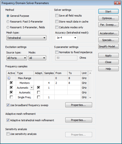
    There are three different methods to choose from.  For the example here, choose the General Purpose frequency domain solver.  In the Mesh Type combo box you may choose between Hexahedral and Tetrahedral Mesh.  Please choose Tetrahedral Mesh.

    S-Parameters in the frequency domain are obtained by solving the field problem at different frequency samples.  These single S-Parameter values are then used by the broadband frequency sweep to get the continuous S-Parameter values.  With the default settings in the Frequency samples frame the number and the position of the frequency samples are chosen automatically in order to fit the required accuracy limit throughout the entire frequency band.

    Unlike the time domain solver, the tetrahedral frequency domain solver should always be used with the Adaptive tetrahedral mesh refinement.  Otherwise, the initial mesh may lead to a poor accuracy.  Therefore, the corresponding check box is activated by default.

    All other settings may also be left unchanged.  Press Start to begin the calculation.

    There may be old results present from the previous transient solver run that will be overwritten when starting a different solver.  In this case, the following warning message appears:

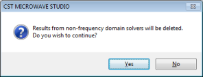
    Press Yes to acknowledge the deletion.  A progress bar and an abort button appear in the status bar showing information about the solver stages. After the desired accuracy for the S-Parameter has been reached, the simulation stops. When the simulation has finished or if it has been aborted, both items disappear again.

    During the simulation, the Message Window will show some details about the performed simulation.

    Results of the Frequency Domain Solver   

    Congratulations, you have simulated the coaxial connector using the frequency domain solver!  Lets review the results:

    1D Results (S-Parameters)

    You can visualize the maximum difference of the S-Parameters for two subsequent passes by selecting 1D Results   Adaptive Meshing  f=8  Delta S from the navigation tree:

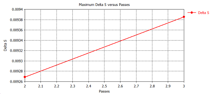
    As evident in the above plot, only three passes of the mesh refinement were required to obtain highly accurate results within the given accuracy level, which is set to 1% by default.

    You can view the S-Parameters by selecting 1D Results > S-Parameters in the navigation tree.

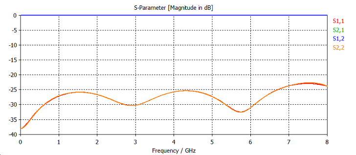
    As expected, the input reflection S1,1 is quite small across the entire frequency range.

    2D and 3D Results (Port Modes and Field Monitors)

    Finally, you can observe the 2D and 3D field results.  You should first inspect the port modes that can be easily displayed by opening the 2D/3D Results  Port Modes  Port1 folder from the navigation tree.  To visualize the electric field of the port mode, please click on the e1 folder.  Open the Select Port Mode dialog box by selecting Results  Select Mode Frequency from the main menu and change the frequency to 4 GHz.  Please confirm your setting by pressing OK.  After properly rotating the view, you should obtain a plot similar to the following picture:

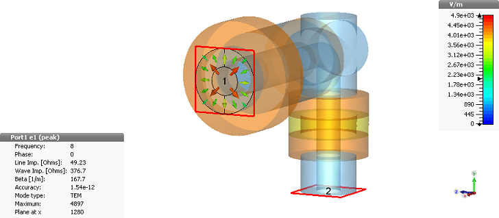
    The plot also shows some important properties of the mode, such as mode type, propagation constant and line impedance.  The port mode at the second port can be visualized in the same manner.

    The three-dimensional h-field distribution can be displayed by selecting one of the entries in the 2D/3D Results  H-Field folder from the navigation tree.  The magnetic field at a frequency of 2 GHz can thus be visualized by clicking at the 2D/3D Results  H-Field  h-field (f=2) [1] entry:

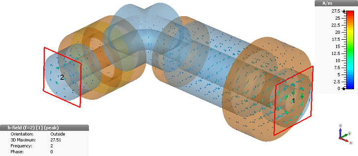
    You can toggle an animation of the currents on and off by selecting Result Tools  2D/3D Plot  Animate Fields.  The surface currents for the other frequencies can be visualized in the same manner, as shown above.

    Comparison of the Solver Results  

    The next plot shows the S-Parameters S1,1 and S1,2 resulting from the time domain and frequency domain simulations.  Plotting the S-Parameter curves in the same graph allows for a better comparison.

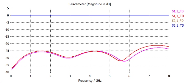
    As you can see, the results agree very well.  Since the results are not converged to the highest possible accuracy level, there is still a slight difference between the curves.  When refining the accuracy limit in the adaptive mesh refinement the difference will become negligible.

上一頁  [1] [2] [3] [4] [5] [6] [7] [8] [9] [10]