


- 1
- 2
- 3
- 4
- ���F(xi��n)�ڵ�λ�ã� ��EDA�W(w��ng) >> CST >> CST�O(sh��)Ӌ(j��)��(sh��)�� >> ����
CST�C��ǻ�w�O(sh��)Ӌ(j��)������CST2013�O(sh��)Ӌ(j��)��(sh��)��
Eigenmode Calculation with AKS
Calculating the Eigenmodes Using Fully Automatic Solver Settings
Please enter the eigenmode solver control dialog box more by pressing Home: Simulation > Start Simulation . Please change the mesh type to hexahedral in the Solver settings frame.
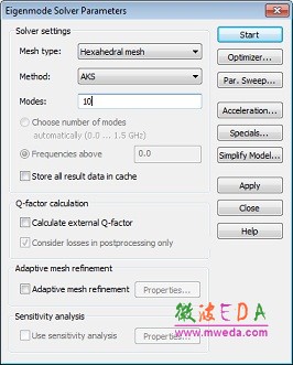
The only setting that commonly needs to be specified here is the number of Modes to be calculated. The solver will then calculate this number of modes starting from the lowest resonance frequency. It is usually advantageous to specify more modes than you are actually searching for. Thus, assuming that you want to calculate the first five modes in this example, you should advise the eigenmode solver to calculate 10 modes. Afterwards, press the Start button to run the simulation.
Due to the Perfect Boundary Approximation®, the number of mesh cells required for discretizing this example is quite small (roughly 7700). This, in fact, corresponds to a system of equations consisting of about 23,100 unknowns. Calculating eigenmodes for such a system takes only a few minutes to complete on a modern PC.
After the solver has finished its work, the resonance frequencies of the first ten modes are displayed in the result window:
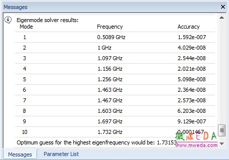
The accuracy for the mode solution is excellent for all the required modes. A mode with an accuracy of less than 1e-3 can usually be considered sufficiently accurate.
In order to review the solver time required to achieve these results, you can display the solver log-file by selecting Simulation: Solver > Logfile . Please scroll down the text to obtain the following timing information (the actual values may vary depending on the speed of your computer):
Mesh generation time : 3 s
Solver time : 8 s
Total time : 11 s
--------------------------------------------------------------
Optimizing the Performance for Subsequent Calculations
To this point, you have successfully calculated the eigenmodes for this device in a reasonable amount of time. However, if you intend to make parametric studies it may be advantageous to speed up the solver for subsequent runs. This performance tuning step is quite simple: The eigenmode solver can make use of a guess for the highest eigenmode frequency you are looking for. The eigenmode solver automatically determines this guess from a previous calculation and prints the result in the log-file. This information is shown right below the timing information:
--------------------------------------------------------------
Optimum guess for the highest eigenfrequency would be: 1.73153
--------------------------------------------------------------
In order to demonstrate how this information can be used for improving the solvers speed, you should now recalculate the eigenmodes to compare the time required for the simulation. Please enter the eigenmode solver control dialog box once more by pressing Home: Simulation > Start Simulation . In this dialog box, press the Specials button in order to open a dialog box for more advanced settings:
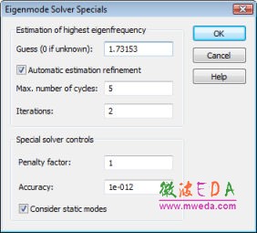
Once you have obtained a guess for the highest eigenfrequency of interest (here 1.73153 GHz), you can enter this value in the Guess field. If you dont know this value, just enter zero to let the solver estimate this value automatically. After pressing the OK button in this dialog box you can restart the eigenmode solver by pressing the Start button.
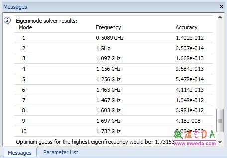
Again, a progress bar will appear informing you of the status of your calculation. Please note that there is no need for recalculating the matrix because the structure has not been changed. The solver will finish its work after a short time, giving the same results as before for the eigenfrequencies. If you now compare the solver times, you can see that specifying the guess for the highest eigenfrequency could speed up the solution process.
Please remember that these steps are only made in order to illustrate how to speed up the solver for parametric sweeps or optimizations. The accuracy of the solution will also be excellent using the fully automatic procedure without this additional setting. For a single analysis of a particular device, this performance tuning is not necessary, but it might further improve the accuracy:
-
CST����ҕ�l�̳̣��Y�(zhu��n)���v�⣬ҕ�l������ʾ���Ļ��A(ch��)�v��ѭ��u�M(j��n)�����Y(ji��)�����¹��̰������������ٌW(xu��)��(x��)����CST���O(sh��)Ӌ(j��)��(y��ng)��...��Ԕ��(x��)��B��
- CST�쾀(xi��n)�O(sh��)Ӌ(j��)���쾀(xi��n)��O(sh��)Ӌ(j��)��CST2013�O(sh��)Ӌ(j��)��(sh��)��
CSTͬ�S��(xi��n)�����ķ����O(sh��)Ӌ(j��)������CST2013�O(sh��)Ӌ(j��)��
ʹ��CST���������M(j��n)��TDRӋ(j��)�����
CST�cMatlab�B���O(sh��)��
CST�������Һ�Agilent ADS �f(xi��)ͬ�����B���O(sh��)��
CST�������Ҳ鿴VSWR�Y(ji��)��
CST��������Y(ji��)������c�ⲿ��(sh��)��(j��)�M(j��n)�б��^
CST�������Ҳ��õ���Ҫ�㷨
ʹ��CST�������ҵĕr(sh��)�����������늴�(w��n)�}��
늴ż��ݵĔ�(sh��)ֵ�����������CST2013
CST�������ܺͷ��漼�g(sh��)
CST�O(sh��)Ӌ(j��)�h(hu��n)�� �� CST2013
���]�n��

-

HFSS�W(xu��)��(x��)��Ӗ(x��n)�n�����b
7������ҕ�l�̳�,2���̲�,�Әӽ�(j��ng)��
-

ADS�W(xu��)��(x��)��Ӗ(x��n)�n�����b
��(gu��)��(n��i)���(qu��n)������(j��ng)���ADS��Ӗ(x��n)�̳����b
-

�����l�����O(sh��)Ӌ(j��)��Ӗ(x��n)�ϼ�
��ȫ��������l�����O(sh��)Ӌ(j��)��Ӗ(x��n)�ϼ�
-

Ansoft Designer �W(xu��)��(x��)��Ӗ(x��n)�n�����b
����Ansoft Designer������Ӗ(x��n)�̲�
-
���y(c��)��?j��)x��ʹ����Ӗ(x��n)�̳�
ʸ�W(w��ng),�l�V�x,��̖(h��o)Դ...,�ӘӾ�ͨ
-

�_(t��i)�����A��W(xu��)���l��(zhu��n)�I(y��)�n�����b
�c�I(y��)���B�Ӿo�ܵ��n��,�W(xu��)������...
-

Les Besser���l��Ӗ(x��n)��(j��ng)��ԭ��ҕ�l
�I(y��)���ţLes Besser����Ӗ(x��n)�n��...
-

PCB�O(sh��)Ӌ(j��)�W(xu��)��(x��)��Ӗ(x��n)�n�����b
Allegro,PADS,PCB�O(sh��)Ӌ(j��),�䌍(sh��)�ܺ�(ji��n)��..
-

Hyperlynx,SIwave,�����QSI��(w��n)�}
-

�h(yu��n)���ھ�(xi��n)��Ӗ(x��n)
�F(xi��n)��(ch��ng)�v��,��(sh��)�r(sh��)����,�����W(xu��)��(x��)�ɲ��`